Tag Archives: RS232

CO2 measurement with SCD30, Arduino and Matlab

Loading

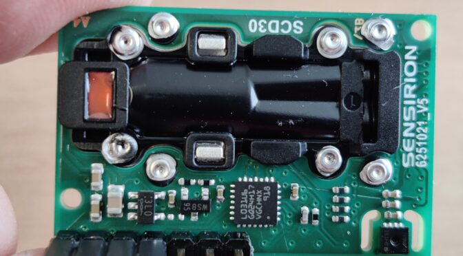
This project – actually a mini project – might also be interesting for one or the other. It is the now well-known and frequently used carbon dioxide sensor SCD30 (CO2 sensor) from the manufacturer Sensirion. There are a number of projects that can be found on the internet. As part of a quick test setup, I tried to read out the data from the sensor using an Arduino Uno board in order to then display it in a plot using the Matlab software. The data transfer takes place via the serial interface or via the serial protocol of the USB-UART.

To connect the SCD30 to the Arduino, you need the power supply and the I²C data bus – so in total just four wires. This means that the minimum configuration is fulfilled and the data can be read out.

The sensor itself works on the principle of NDIR technology. (NDIR = non-dispersive-infrared). That means the sensor is a small spectrometer. The medium to be examined is fed into a sample chamber. The sample chamber is illuminated by an infrared source and the IR light shines through the medium and a very narrow-band wavelength filter and then hits the IR detector. The wavelength of the filter is designed in such a way that precisely those wavelengths are let through that are absorbed by the molecules of the medium (gas). Depending on the number of molecules or the density of the gas, fewer light beams are recognized by the detector. A second measuring chamber, which is filled with a reference gas, serves as a reference. A controller on the sensor evaluates this information and forwards it in the form of ppm via the I²C (or switchable MOD-Bus) interface. There is also a temperature and humidity sensor on the board, the data of which can also be read out via the bus. The preset I²C address of the SCD30 is 0x61. The exact information on the data protocol can be found in the documentation from Sensirion.

Ideally, as almost always, there is already a ready-made library suitable for students for the various microcontrollers. So you don’t have to worry anymore and can read out the data from the connected sensor directly. The example programs can be found under the examples of the libraries.

electrical specifications

The Arduino with 3.3V or 5V can be used for the supply voltage of the sensor. However, caution is advised when using the I²C bus: Here the input high level is set at 1.75-3.0V and the output high level with a maximum of 2.4V. But on an Arduino the levels are 5V !! So a level shifter has to be built in here – or at least, suitable resistors for a quick test.

The program code listed here essentially comes from the example of the library by Nathan Seidle from SparkFun Electronics:

 1
 2
 3
 4
 5
 6
 7
 8
 9
10
11
12
13
14
15
16
17
18
19
20
21
22
23
24
25
26
27
28
29
30
31
32
33
34
35
36
37
38
39
40
/*
By: Nathan Seidle SparkFun Electronics  
Library: http://librarymanager/All#SparkFun_SCD30  
*/

#include <Wire.h>
#include "SparkFun_SCD30_Arduino_Library.h" 
SCD30 airSensor;

void setup()  
{
  Wire.begin();
  Serial.begin(9600);
  //Serial.println("SCD30 Example");
  airSensor.begin(); //This will cause readings to occur every two seconds
}

void loop()  
{
  if (airSensor.dataAvailable())
  {
   // Serial.print("co2(ppm):");
   
    Serial.print(airSensor.getCO2());

    //Serial.print(" temp(C):");
    Serial.print(",");
    Serial.print(airSensor.getTemperature(), 1);

   // Serial.print(" humidity(%):");
    Serial.print(",");
    Serial.print(airSensor.getHumidity(), 1);

    Serial.println();
  }
  else
    //Serial.println("No data");

  delay(500);
}


With these lines of code in the Arduino Uno and the correct wiring (SDA -> to Arduino A4 and SCL -> to Arduino A5 via a suitable level converter) you can continue with Matlab. The Arduino should now output the following lines in a serial terminal: (example)

473,28.5,12.9
473,28.5,13.0
470,28.5,13.1
469,28.5,12.9
466,28.5,12.9
465,28.5,12.7
465,28.5,12.5
463,28.6,12.6
461,28.6,12.5
463,28.5,12.4 … und so weiter

This now has to be read into Matlab and recorded over a definable period and at the same time displayed in a plot. The matlab script here makes it possible … (pn if someone needs it)

The result is a plot that shows the course of CO2 in the room (in this case on my office desk).


Long-term measurements with Keithley and Matlab

Loading

Keithley2000 desk multimeter

The bench multimeter from Keithley is an old companion in the field of measuring instruments. The types of the 2000 series are predominantly used in our laboratories. They are available in different equipment variants with regard to the interfaces to the outside world. Here GBIP bus is of course a standard, as is RS232. The newer devices now have a LAN interface with which communication via the Internet protocol is possible. Each of these interfaces can be used to communicate with the device using “Standard Commands for Programmable Instruments” (SCPI). In this example I will control the Keithley 2000 via Matlab and read out measured values ​​cyclically over a longer period of time, save them in Matlab and finally output them in a plot – virtually configure a simple data logger. The purpose of this setup is to record the voltage curve (or current) of a rechargeable battery or battery of a low-energy device.

backside of the Keithley 2000
GPIB Interface (IEEE488)
RS232 interface

In this example I will use the serial data transmission via the classic RS232 interface, as this is completely sufficient for my application. In addition, I can save myself the installation of the driver packages for the GPIP-USB interface. 🙂 Since many of the current computers and laptops no longer have any RS232 ports, a USB-RS232 adapter (e.g. FTDI232 etc.) is required.

USB-RS232 Adaper am Keithley2000

Once the connection between the multimeter and the computer has been established, communication can take place via a Matlabscript, as in this example. The Keithley only needs to be told that it should “talk” over the serial interface. The following code snippets show how you can easily read out data via SCPI:


serialObject = instrfind('Type', 'serial', 'Port', 'COM26', 'Tag', '');
%serialPort = 'COM23';
%serialObject = serial(serialPort,'BaudRate',9600, 'DataBits',8);

if isempty(serialObject)
serialObject = serial('COM26','BaudRate',57600, 'DataBits',8);
else
fclose(serialObject);
serialObject = serialObject(1)
end

%%%%%%%%%%%%%%%%%%%%%%%%%%%%%%%%%%%%%%%%%%%%%%%%%%%%%%%
%
% Sourcemeter 2000 setup
%
%%%%%%%%%%%%%%%%%%%%%%%%%%%%%%%%%%%%%%%%%%%%%%%%%%%%%%
fopen(serialObject)
% fprintf(serialObject,':*RST')

time = now;
voltage = 0;
%%
figureinstanz = figure('NumberTitle','off',...
'Name','Spannungslogg',...
'Color',[0 0 0],'Visible','off');
plotinstanz = plot(voltage,time,'Color','red');

%% Messzeit und evtl Messintervall
stoptime = 10; %60 seconds
timeInterval = 1; % brauch' ma jetzt nicht

% Messgeraet einstellen
fprintf(serialObject,':SOUR:FUNC:MODE CURR'); % current source selection.
fprintf(serialObject,':SOUR:CURR:MODE FIXED'); % changes voltage mode to fixed
fprintf(serialObject,':SOUR:CURR:LEV 0'); % sets current to 0

fprintf(serialObject,':SENS:FUNC &quot;VOLT&quot;');
fprintf(serialObject,':SENS:VOLT:PROT 4');
%fprintf(serialObject,':SENS:CURR:RANG:AUTO ON');
fprintf(serialObject,':SENS:VOLT:RANG 10');
fprintf(serialObject,':FORM:ELEM VOLT');

% %fprintf(serialObject,':TRAC:COUN 1');
% %fprintf(serialObject,':TRAC:FEED:CONT NEV');
%
%
% fprintf(serialObject,':TRAC:CLE');
%
% fprintf(serialObject,':TRAC:POIN 10');
% fprintf(serialObject,'TRAC:FEED:SENS');
% fprintf(serialObject,'TRAC:FEED:CONT NECT');
% fprintf(serialObject,'TRIG:COUN 10');
% fprintf(serialObject,':OUTP ON');
%
% fprintf(serialObject,':INIT');
% fprintf(serialObject,':TRACE:DATA?');

%% Daten abholen
count = 1; voltage(1)=4
tic;
time=toc;
% while time&lt;=stoptime
while voltage&gt;=1.5
% fprintf(serialObject,':INIT');
% fprintf(serialObject,':TRAC:FEED SENS');
% fprintf(serialObject,':TRAC:DATA?');
%
fprintf(serialObject,':READ?');
voltage(count) = fscanf(serialObject,'%f');
time(count) = toc;
set(plotinstanz,'YData',voltage,'XData',time);
set(figureinstanz,'Visible','on');
pause(timeInterval);
count = count +1;
end

figure(1);
plot(time,voltage);
grid on; hold on;
xlabel('Zeit [s]'); ylabel('Batteriespannung [V]')
title('Spannungsverlauf Batterie 3V Lithium (2032 mit Modul) im default mode');

% fprintf(serialObject,':OUTP OFF');
%% Put the instrument in local mode
fprintf(serialObject,'SYSTEM:LOCAL');
fclose(serialObject);

The following plot shows what such a data log looks like. Here, the voltage curve of a nearly discharged battery is recorded over time until the consumer is switched off.