Tag Archives: GPIB

Long-term measurements with Keithley and Matlab

Loading

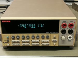
Keithley2000 desk multimeter

The bench multimeter from Keithley is an old companion in the field of measuring instruments. The types of the 2000 series are predominantly used in our laboratories. They are available in different equipment variants with regard to the interfaces to the outside world. Here GBIP bus is of course a standard, as is RS232. The newer devices now have a LAN interface with which communication via the Internet protocol is possible. Each of these interfaces can be used to communicate with the device using “Standard Commands for Programmable Instruments” (SCPI). In this example I will control the Keithley 2000 via Matlab and read out measured values ​​cyclically over a longer period of time, save them in Matlab and finally output them in a plot – virtually configure a simple data logger. The purpose of this setup is to record the voltage curve (or current) of a rechargeable battery or battery of a low-energy device.
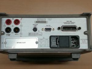
backside of the Keithley 2000
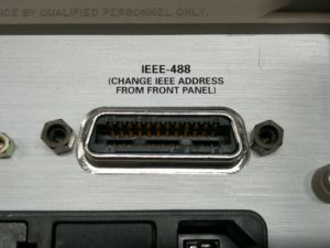
GPIB Interface (IEEE488)
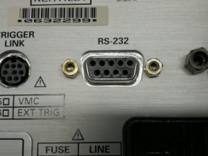
RS232 interface

In this example I will use the serial data transmission via the classic RS232 interface, as this is completely sufficient for my application. In addition, I can save myself the installation of the driver packages for the GPIP-USB interface. 🙂 Since many of the current computers and laptops no longer have any RS232 ports, a USB-RS232 adapter (e.g. FTDI232 etc.) is required.
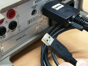
USB-RS232 Adaper am Keithley2000

Once the connection between the multimeter and the computer has been established, communication can take place via a Matlabscript, as in this example. The Keithley only needs to be told that it should “talk” over the serial interface. The following code snippets show how you can easily read out data via SCPI:


serialObject = instrfind('Type', 'serial', 'Port', 'COM26', 'Tag', '');
%serialPort = 'COM23';
%serialObject = serial(serialPort,'BaudRate',9600, 'DataBits',8);

if isempty(serialObject)
serialObject = serial('COM26','BaudRate',57600, 'DataBits',8);
else
fclose(serialObject);
serialObject = serialObject(1)
end

%%%%%%%%%%%%%%%%%%%%%%%%%%%%%%%%%%%%%%%%%%%%%%%%%%%%%%%
%
% Sourcemeter 2000 setup
%
%%%%%%%%%%%%%%%%%%%%%%%%%%%%%%%%%%%%%%%%%%%%%%%%%%%%%%
fopen(serialObject)
% fprintf(serialObject,':*RST')

time = now;
voltage = 0;
%%
figureinstanz = figure('NumberTitle','off',...
'Name','Spannungslogg',...
'Color',[0 0 0],'Visible','off');
plotinstanz = plot(voltage,time,'Color','red');

%% Messzeit und evtl Messintervall
stoptime = 10; %60 seconds
timeInterval = 1; % brauch' ma jetzt nicht

% Messgeraet einstellen
fprintf(serialObject,':SOUR:FUNC:MODE CURR'); % current source selection.
fprintf(serialObject,':SOUR:CURR:MODE FIXED'); % changes voltage mode to fixed
fprintf(serialObject,':SOUR:CURR:LEV 0'); % sets current to 0

fprintf(serialObject,':SENS:FUNC "VOLT"');
fprintf(serialObject,':SENS:VOLT:PROT 4');
%fprintf(serialObject,':SENS:CURR:RANG:AUTO ON');
fprintf(serialObject,':SENS:VOLT:RANG 10');
fprintf(serialObject,':FORM:ELEM VOLT');

% %fprintf(serialObject,':TRAC:COUN 1');
% %fprintf(serialObject,':TRAC:FEED:CONT NEV');
%
%
% fprintf(serialObject,':TRAC:CLE');
%
% fprintf(serialObject,':TRAC:POIN 10');
% fprintf(serialObject,'TRAC:FEED:SENS');
% fprintf(serialObject,'TRAC:FEED:CONT NECT');
% fprintf(serialObject,'TRIG:COUN 10');
% fprintf(serialObject,':OUTP ON');
%
% fprintf(serialObject,':INIT');
% fprintf(serialObject,':TRACE:DATA?');

%% Daten abholen
count = 1; voltage(1)=4
tic;
time=toc;
% while time<=stoptime
while voltage>=1.5
% fprintf(serialObject,':INIT');
% fprintf(serialObject,':TRAC:FEED SENS');
% fprintf(serialObject,':TRAC:DATA?');
%
fprintf(serialObject,':READ?');
voltage(count) = fscanf(serialObject,'%f');
time(count) = toc;
set(plotinstanz,'YData',voltage,'XData',time);
set(figureinstanz,'Visible','on');
pause(timeInterval);
count = count +1;
end

figure(1);
plot(time,voltage);
grid on; hold on;
xlabel('Zeit [s]'); ylabel('Batteriespannung [V]')
title('Spannungsverlauf Batterie 3V Lithium (2032 mit Modul) im default mode');

% fprintf(serialObject,':OUTP OFF');
%% Put the instrument in local mode
fprintf(serialObject,'SYSTEM:LOCAL');
fclose(serialObject);

The following plot shows what such a data log looks like. Here, the voltage curve of a nearly discharged battery is recorded over time until the consumer is switched off.

Read LCR meter via Matlab

Loading

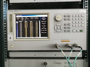
LCR-Meter 4297A Agilent

In this post I would like to devote myself to something else. It’s not about retro technology, it’s about a little thing that makes working in the office/lab easier. One of the many measuring devices I deal with is an old Agilent LCR meter. As is known, the LCR Meter 4297A can be used to measure the inductance, capacitance, etc. of electrical components and generally of structures which are assigned to the electronics / electrical engineering sector. Roughly speaking, the 4297A actually only measures current / voltage, the phase relationship between the two and the energy direction. And at a certain frequency. All parameters such as L, C, R, X, Y, Q, PHI, … are then mathematically calculated and output from these parameters. The frequency here can be set from 1MHz to 3GHz (in 100kHz steps). Ideally, the measuring device can measure not only in one frequency point, but also in many. By “many” is meant here that the measuring device can generate frequency tables with 32 entries. There are eight of these tables. This makes it possible to display the course of a measured variable in the form of a curve. However, this is quite cumbersome. The contents of the tables must be exported and saved manually (as “csv” files) table by table. This means that each table must be selected individually. Then select the “Export List View” dialog – then specify a storage path and file name. Only now are the first 32 records exported. This process must be repeated eight times in total. It is saved on a 3.5 inch floppy disc – the only available medium. You could also hang the 4297A optiona on a LAN and set up file sharing. However, manual export is not spared. The .csv files can now be opened on a “normal” computer. They must then be put together manually in postprocessing. Only now can a diagram be made from the data. Here Matlab from Matworks is a good tool, which is often used in our laboratories as part of training.

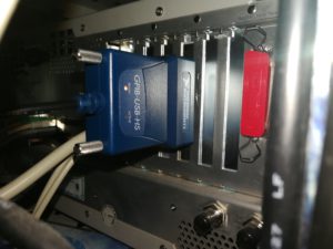
NI GPIB – USB Controller

To simplify this cumbersome process considerably, I created a small script that communicates with the measuring device using the SCPI commands (Standard Commands for Programmable Instruments). That means: The measuring device is connected to a PC via a GPIB-USB controller. A Matworks Matlab installation including the required toolboxes is located on the PC. The Matlab script should now simply switch through the tables in sequence and read out the contents of the individual parameters and save them in an array. The content of the arrays is then displayed directly in a plot. However, this method only uses the contents of the tables. It would of course also be possible to set any desired frequency directly in a loop using the script, read out the measured values, select the next frequency, etc. This would max. Total 29990 points over the entire frequency range. The eight tables, each with 32 points, only allow 256 points. For now, however, that is sufficient and also much faster.

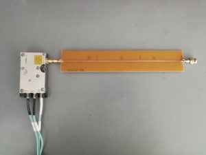
Transmission Line 50 Ohm termination resistor
line is terminated

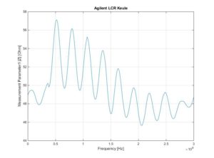
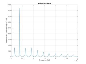
The example shows the impedance curve (Z curve) of a 50 Ohm transmission line. The end of the line is terminated with a 50 ohm resistor. The frequency range is 1MHz to 3 GHz. The situation is different if the line is open or closed briefly. The electromagnetic wave is then not converted into thermal energy at the end of the line, as in the “matched” system, but is reflected back into the system.

line is shortened

The following very simple Matlabscript enables the reading of the measuring device parameters. The script serves as an example of how to get the measurement data quickly. The programming manual of the manufacturer of the LCR meter lists all SCPI commandos and plenty of examples with which you can communicate with the measuring device.


%auslesen der agilent LCR Keule 4287A
%gekodet von ingmar bihlo Ende November 2017

%anschluss über gpib ni adapter
%LCR gpip adresse: 5
%%
%vorarbeiten an LCR Keule
%
% Es müssen 8 Tabellen mit je 32 Punkten definiert sein
% (power und average ist egal, wird nicht ausgelesen)
% die CALibration muss gemacht worden sein
% unter "measurement parameters" muessen vier parameter definiert sein
% zb. Z, qhi, R, L, etc... diese sind dann in den variablen param1 bis 4
% enthalten

%%

% gpib interface oeffnen und identifier lesen
g = gpib('ni', 0, 5);
g.InputBufferSize = 100000; % Set the buffer size
fopen(g);
fprintf(g, '*IDN?')
idn = fscanf(g);
fclose(g);

num1all=0; % initialisieren der variablen für den summenvector
num2all=0;
num3all=0;
num4all=0;
freq=0;

fopen(g);
%read list parameters (frequency points)
fprintf(g, ':SOUR:LIST?');
fpoint=fscanf(g);
listchar=strsplit(fpoint,',');
list=[cellfun(@str2num, listchar(:,1:end))]
clear listchat; clear fpoint;

%analyze list content
points=freq(1);

for i=1:8
%Tables selecten
fprintf(g, strcat(':SOUR:LIST:TABL 0',num2str(i)));
pause(1); %pause 1s zum umschalten der tabelle

%parameter1 abholen
fprintf(g, ':DATA:FDAT1?'); %parameter 1 anfragen
par1=fscanf(g); %parameter 1 holen

string1=strsplit(par1,','); %parameter 1 string nach komma zerlegen
%num1=[cellfun(@str2num, string1(:,1:end))] %parameter 1 strings in dec konvertieren
num1=[cellfun(@str2num, string1(:,1:end))];
num1all=[num1all,num1]; %parameter1 aktuell mit parameter1 aus vorherigem durchlauf concentenaten

fprintf(g, ':DATA:FDAT2?');
par2=fscanf(g);
string2=strsplit(par2,',');
num2=[cellfun(@str2num, string2(:,1:end))]
num2all=[num2all,num2];

fprintf(g, ':DATA:FDAT3?');
par3=fscanf(g);
string3=strsplit(par3,',');
num3=[cellfun(@str2num, string3(:,1:end))]
num3all=[num3all,num3];

fprintf(g, ':DATA:FDAT4?');
par4=fscanf(g);
string4=strsplit(par4,',');
num4=[cellfun(@str2num, string4(:,1:end))]
num4all=[num4all,num4];

%read list parameters (frequency points)
fprintf(g, ':SOUR:LIST?');
fpoint=fscanf(g);
listchar=strsplit(fpoint,',');
listraw=[cellfun(@str2num, listchar(:,1:end))];
list=listraw(:,2:end); %von pos2 das feld schreiben (an pos ist die anzahl der zeilen)

for c=1:3:96
freq=[freq,list(c)]; %von jedem 3. wert aus list ein neues array bilden
end

clear listchat; clear fpoint;

pause (1);
end

%%

%ausgabevariablen festlegen
frequency=freq(:,2:end);
param1=num1all(:,2:end);
param2=num2all(:,2:end);
param3=num3all(:,2:end);
param4=num4all(:,2:end);

%%
% Cell array richtig uma drahn
x1=param1(1:32);
y1=param1(33:256);
param1 = [y1 x1];

x2=param2(1:32);
y2=param2(33:256);
param2 = [y2 x2];

x3=param3(1:32);
y3=param3(33:256);
param3 = [y3 x3];

x4=param4(1:32);
y4=param4(33:256);
param4 = [y4 x4];
%%
%uerberflüssige variablen loeschen
clear c; clear i; clear list; %clear freq;
clear par1;clear par2;clear par3;clear par4;
clear string1;clear string2;clear string3;clear string4;
clear num1all;clear num2all;clear num3all;clear num4all;

fclose(g);

%plotten der ergebnisse
figure(1);
plot(frequency,param1);
grid on; hold on;
xlabel('Frequency [Hz]'); ylabel('Measurement Parameter1 |Z| [Ohm]');
title('Agilent LCR Keule');

figure(2);
plot(frequency,param2);
grid on; hold on;
xlabel('Frequency'); ylabel('Measurement Parameter2');
title('Agilent LCR Keule');

figure(3);
plot(frequency,param3);
grid on; hold on;
xlabel('Frequency'); ylabel('Measurement Parameter3');
title('Agilent LCR Keule');

figure(4);
plot(frequency,param4);
grid on; hold on;
xlabel('Frequency'); ylabel('Measurement Parameter4');
title('Agilent LCR Keule');